A Glioma Brain Digital Twin

From multimodal MRI and brain mechanics to postoperative cognition: a single-patient proof-of-concept

Arvid Lundervold, BSc, MD, PhD · University of Bergen

October 2026

Who this presentation is for

Written for neuro-oncologists, neurosurgeons, clinical neuroscientists and neuropsychologists.

  • Each section opens with a clinical question.
  • Green boxes say why it matters clinically. Orange boxes say what the evidence does not show.
  • The mathematics sits in optional deep-dive slides (press ↓ where shown).
  • Dotted-underlined terms show a definition when you hover over them. There is also a glossary at the end.

Navigation: ← → between sections · ↓ for deep dives · M menu · O overview · F full screen · S speaker notes

Research prototype, not for clinical use.
The results come from one patient (sub-PAT16, open OpenNeuro data). This is a working methods demonstration, not a validated predictive tool. It is not a medical device.

Code, data and notebooks (open):
github.com/arvidl/glioma-brain-digital-twin-public

Nine clinical questions

  1. What is a brain digital twin, and what data do we have?
  2. What do the CANTAB tests measure, and how did the patient change?
  3. What does the brain look like before and after surgery?
  4. How is white matter organised, and how is structural connectivity disrupted?
  5. How do spontaneous brain dynamics change after surgery?
  6. How does the brain deform when the tumour is removed?
  7. How do mechanics modulate neural dynamics?
  8. Does predicted disruption match observed cognitive change?
  9. What would it take to make this clinically useful?

1 · The idea and the data

Why glioma needs more than a tumour map

  • Gliomas are the most common primary malignant brain tumours. Diffuse gliomas (WHO grades 2–4) infiltrate tissue, which blurs the tumour–brain boundary.
  • Surgery balances extent of resection against functional preservation.
  • Postoperative cognition varies widely between patients. It depends on distant network effects and mass-effect release, not only on the lesion site.
  • Mechanical compression from space-occupying tumours can itself harm neurons. Experimental work links chronic compression to neuronal apoptosis and reduced network activity (Zarodniuk et al. 2026).

Clinical question: can we model, for an individual patient, which functions are at risk and why, before and after surgery?
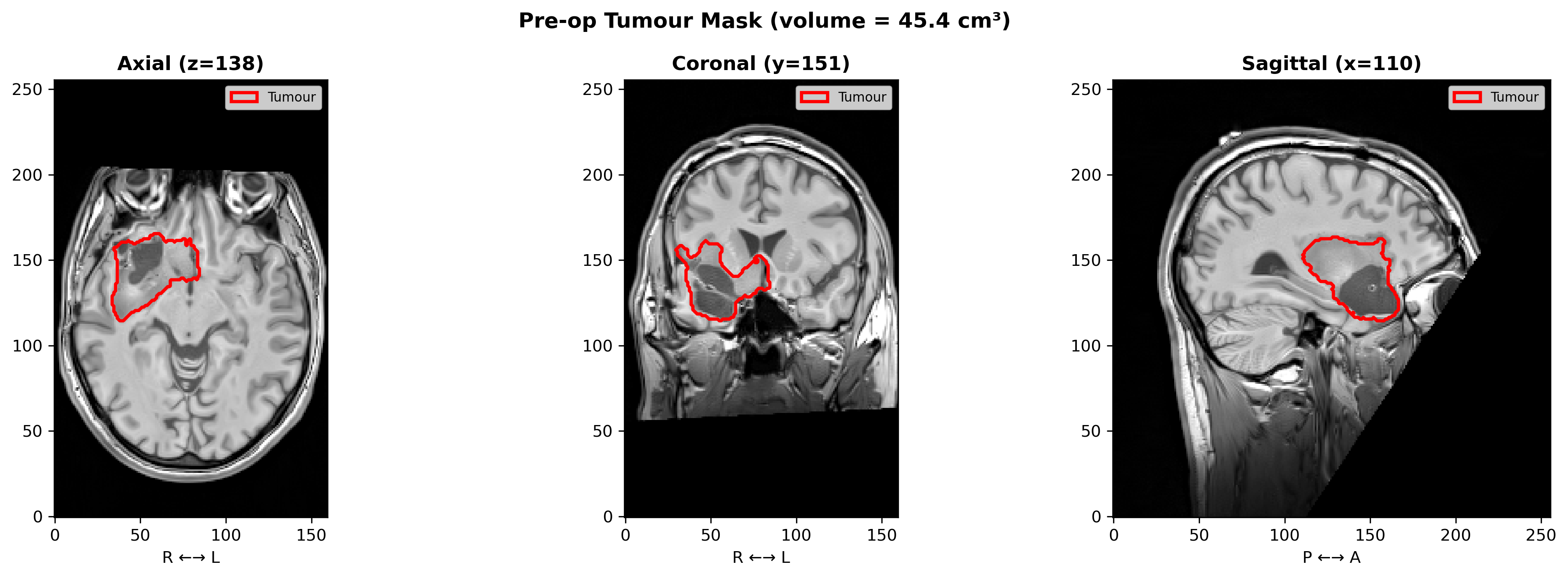
Pre-operative T1-weighted MRI with tumour outline

sub-PAT16: pre-operative tumour outline (red), right fronto-temporal/insular, ≈45 cm³ on the segmentation mask.

What is a brain digital twin?

A patient-specific computational replica that links what we can measure (MRI, cognition) with what we can model (tissue mechanics, network dynamics). It is used to explore what happens if.
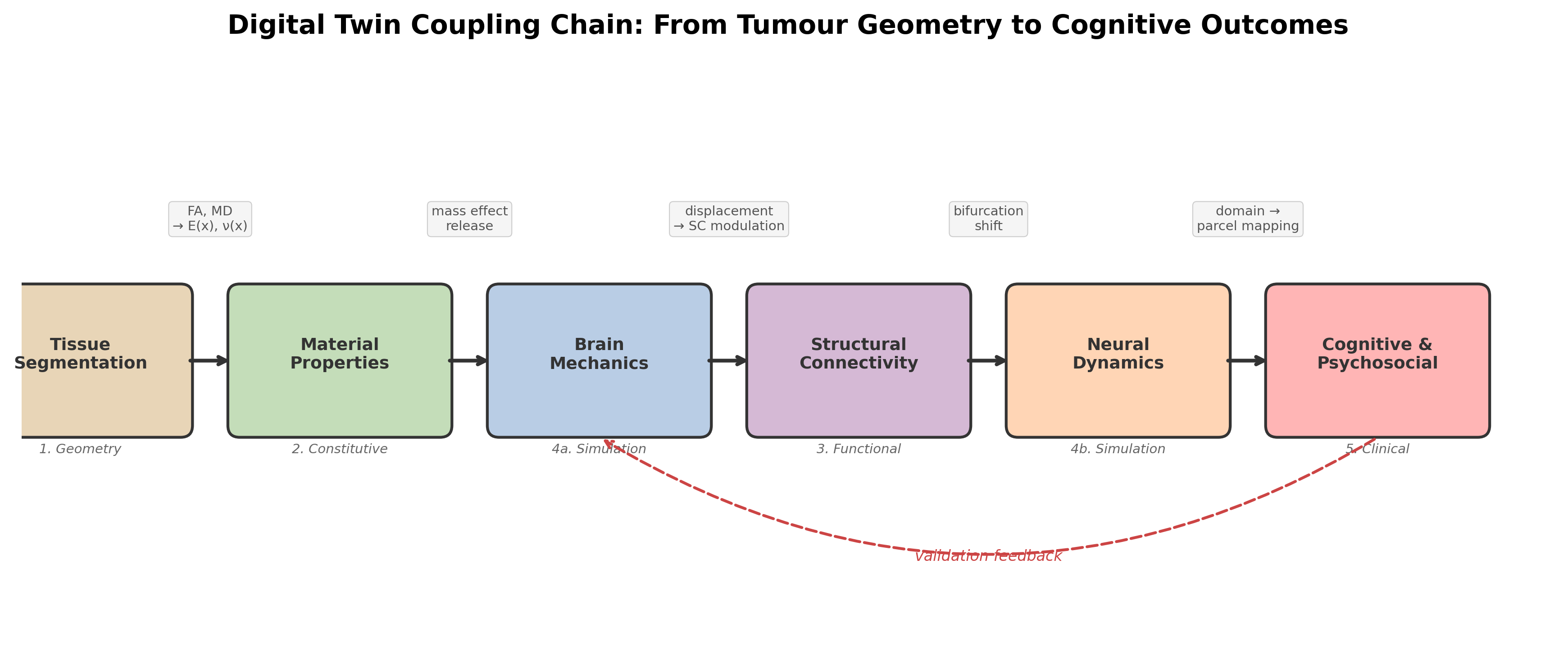
Coupling chain from tissue segmentation to cognitive outcome

The chain ends in cognition and psychosocial state, the outcomes patients care about. That last link is what lets clinical data test the model.

Today’s twin is a one-off, retrospective reconstruction. It is not yet continuously updated with new data, and it is not used for prediction in practice.

The patient and the data

sub-PAT16
Sex, age Male, 39
Diagnosis (as labelled in the dataset) Anaplastic astrocytoma, WHO II–III
Location Right fronto-temporal / insular
Tumour volume 45–50 cm³
Scanner Siemens TrioTim 3 T
Sessions Pre-op and post-op

Open data: Brain Tumor Connectomics, OpenNeuro ds001226 / ds002080, CC0 licence (Aerts et al. 2018, 2022). The diagnosis uses pre-2021 WHO terminology. Molecular markers (such as IDH status) are not available.
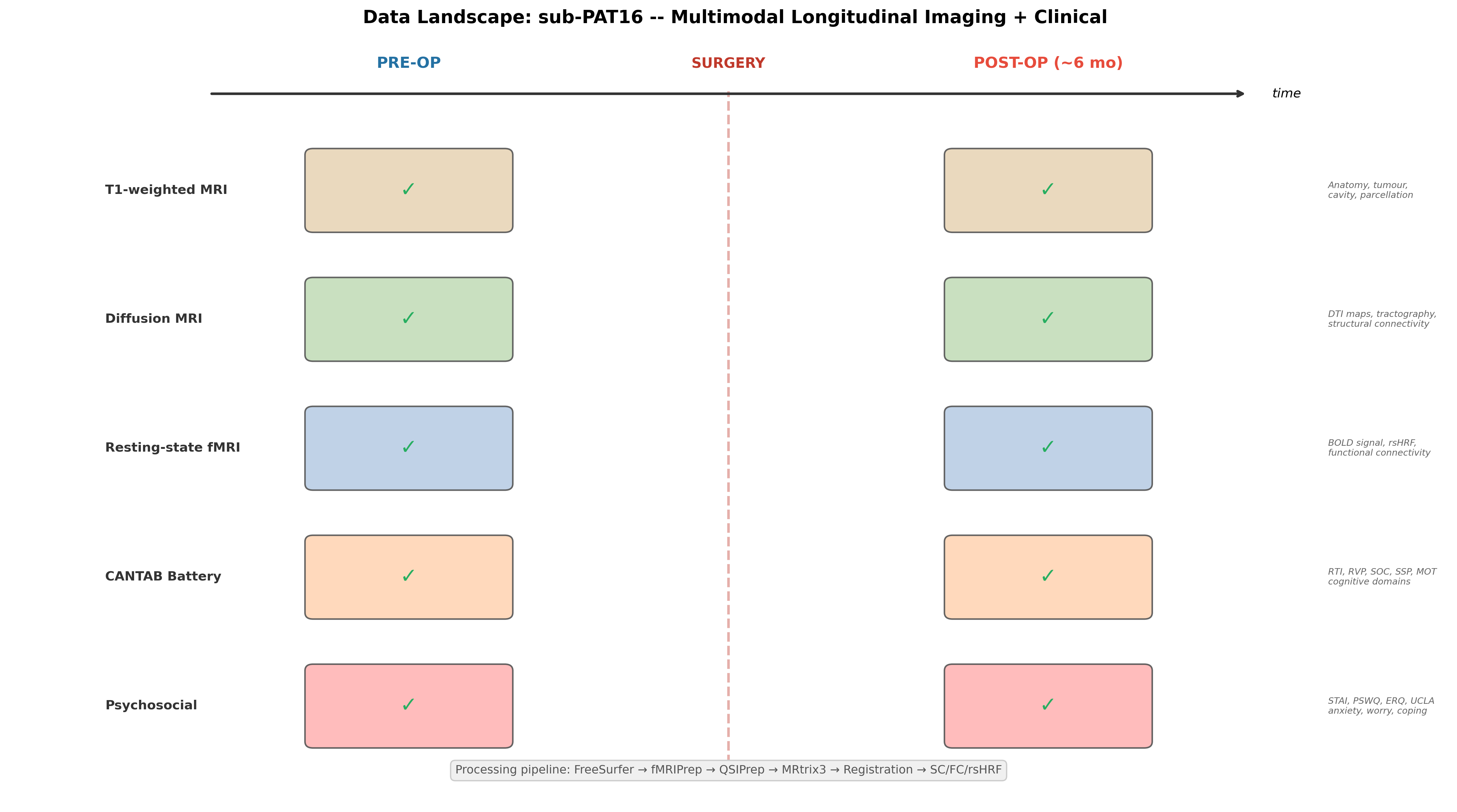
Timeline of imaging and clinical data before and after surgery

The same five data types are available before and after surgery: T1w MRI, diffusion MRI, resting-state fMRI, CANTAB, and psychosocial questionnaires. That pairing is what makes the case useful for testing a twin.

2 · Cognition and psychosocial state

CANTAB: what was measured

Test Domain Main circuits Metric (better =)
MOT Motor screening Basic motor response precentral, paracentral latency (lower)
RTI Reaction time Processing speed, attention precentral, superior frontal, basal ganglia–thalamocortical RT (lower)
RVP Rapid visual processing Sustained attention dorsolateral PFC, inferior parietal A′ (higher)
SOC Stockings of Cambridge Planning, executive dorsolateral PFC, pars opercularis min-move solutions (higher)
SSP Spatial span Visuospatial working memory caudal middle frontal, superior parietal, precuneus span (higher)

Raw scores only. There are no normative z-scores, and there is one pre-op and one post-op session. Practice effects and test–retest variability are not modelled.

How PAT16 changed (interactive)

Psychosocial context changed too (interactive)

  • STAI anxiety 36 → 30 (better)
  • PSWQ worry 54 → 61 (near threshold 62)
  • ERQ reappraisal 24 → 14 (less adaptive coping)
  • UCLA loneliness 40 → 50
  • Employment: employed → sick leave

Worry, coping and isolation affect attention and executive performance independently of the lesion (Eysenck et al. 2007; Gross 2015).

3 · Anatomy before and after surgery

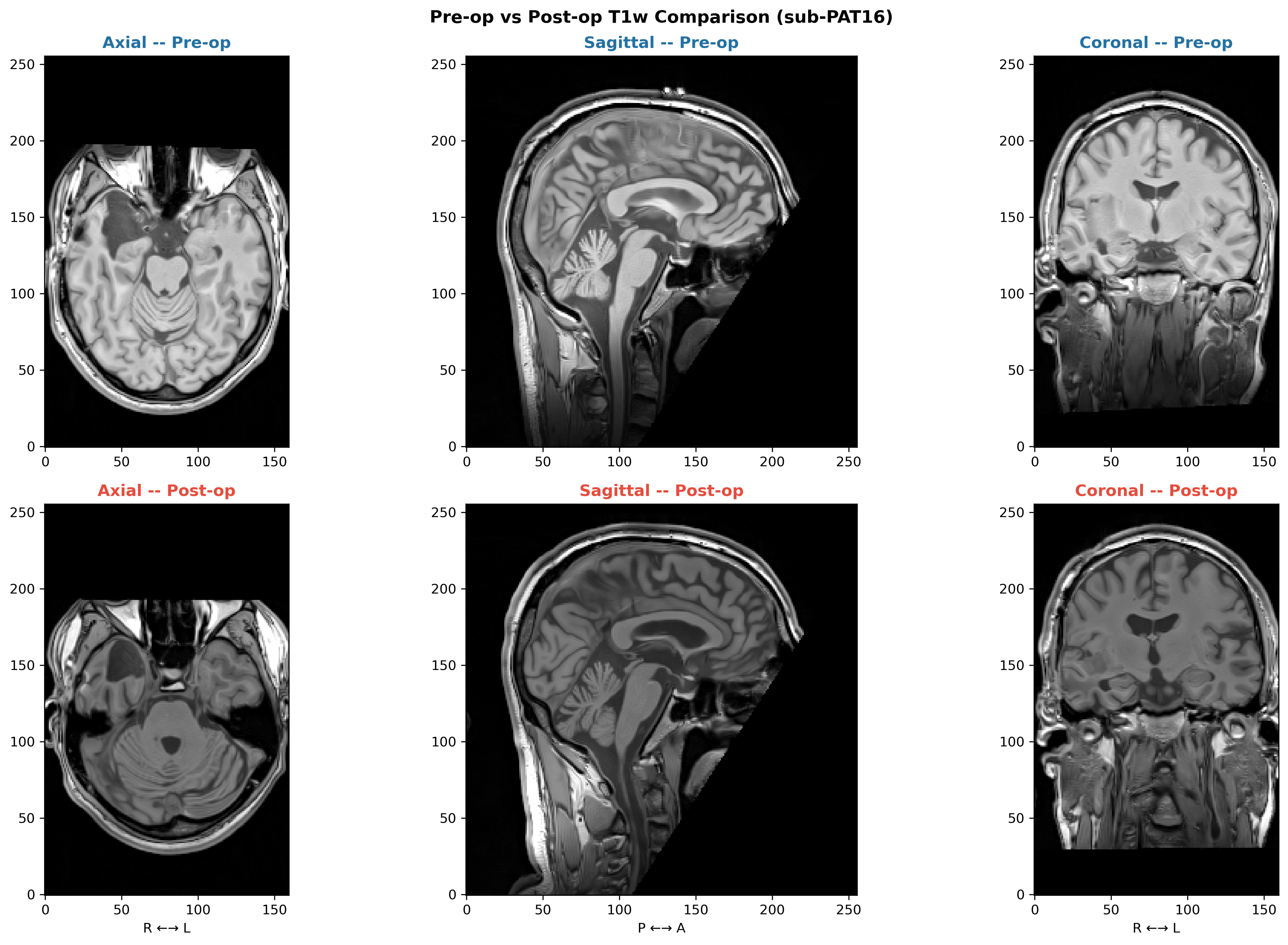
Pre-op vs post-op structural MRI

Pre- and post-operative T1-weighted MRI in three planes

Resection cavity in the right temporal/insular region. Registering the post-op scan to the pre-op scan gives a measured displacement field, which is the “ground truth” the mechanics model is later compared against.

Segmentation and parcellation in practice

Pre-op FreeSurfer segmentation and Desikan–Killiany parcellation in Freeview. These 68 cortical regions are the nodes of the network model.

4 · White matter and structural connectivity

Tractography around the tumour

  • Diffusion MRI → fibre orientation → whole-brain tractography
  • Streamlines are counted between 68 cortical regions, giving the structural connectome (SC)
  • The tumour (yellow) sits next to temporal–insular and fronto-temporal pathways

Tractography near tumour and oedema is biased. Pathways may be missed or invented.

Diffusion → tissue properties → connectome
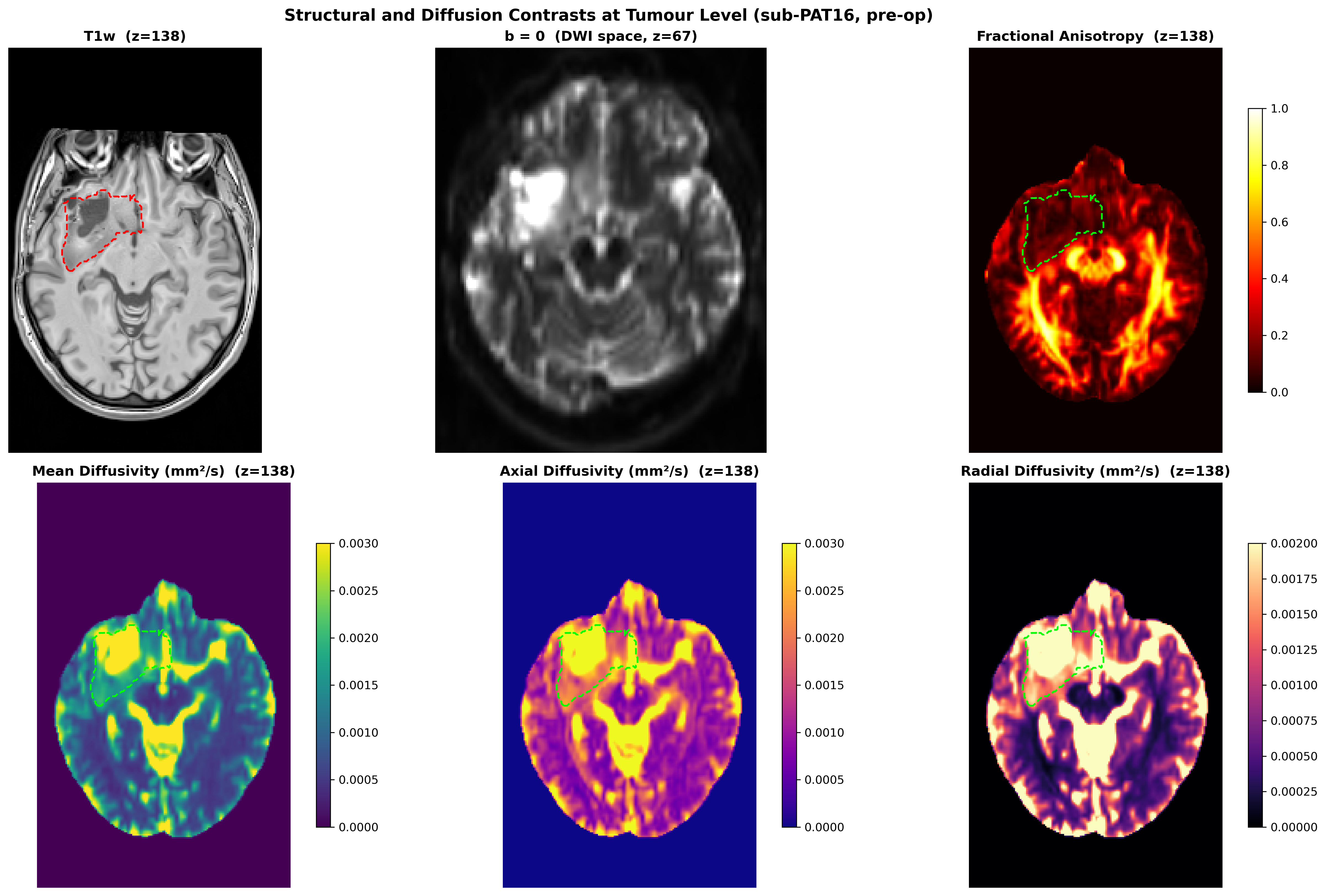
DTI scalar maps

FA and MD maps also inform the tissue stiffness used in the mechanics model.
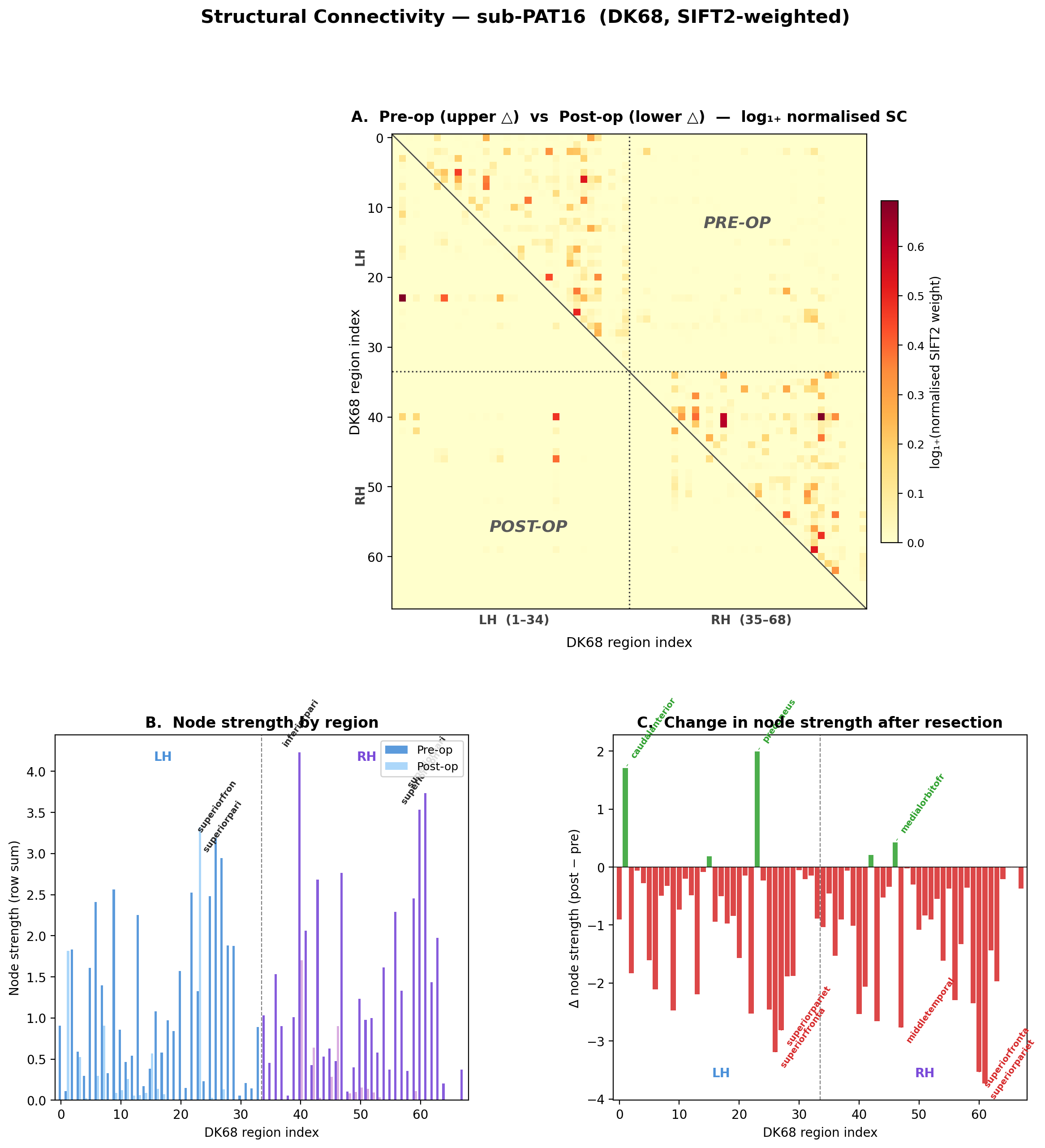
Structural connectivity matrix

68×68 structural connectivity, the network on which the dynamics model runs.

5 · Spontaneous brain dynamics

Resting-state fMRI: the brain’s spontaneous activity

  • Each voxel has a BOLD time course (TR 2.4 s, 180 volumes, 3 mm voxels).
  • Correlating regional time courses gives functional connectivity (FC).
  • A single 55 µl fMRI voxel contains about 5.5 million neurons and 220 km of axons (Logothetis 2008). FC is a very coarse view of the network.

BOLD is an indirect, haemodynamic signal. The tumour and the surgery can change neurovascular coupling itself.

Functional connectivity before surgery
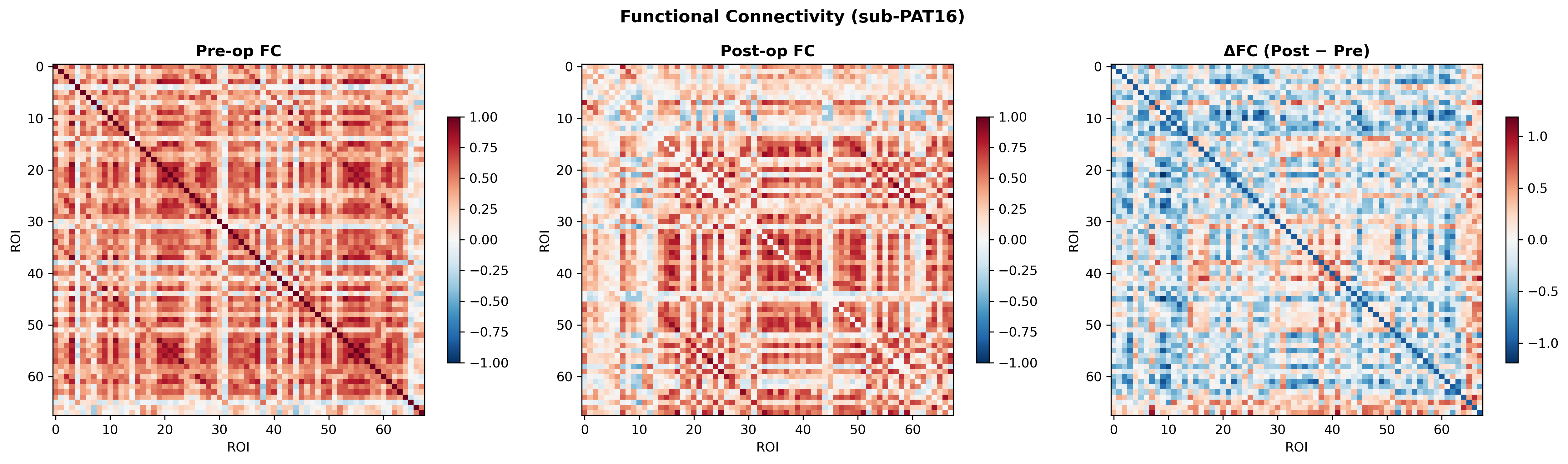
Functional connectivity matrices

Empirical FC is the “target” a whole-brain model should reproduce.

6 · Brain mechanics

How does the brain deform when the tumour is removed?

  • A finite-element model (FEniCSx) of the patient’s brain:
    • geometry from MRI segmentation
    • stiffness modulated voxel by voxel by diffusion MRI
    • loads: gravity plus release of tumour mass effect
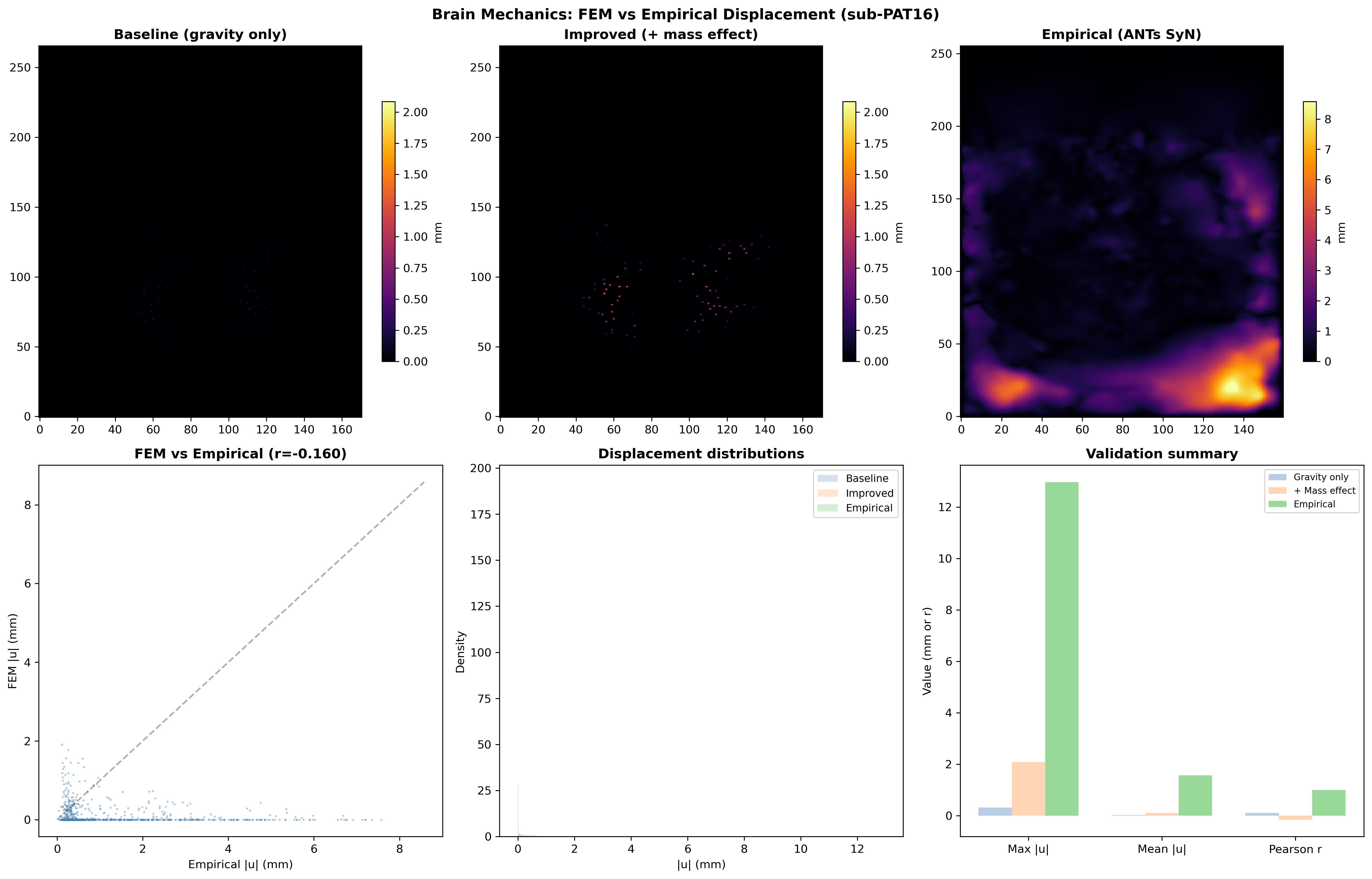
  • Output: a predicted displacement field, compared with the displacement measured by image registration.

Interactive 3D patient geometry: drag to rotate, scroll to zoom, click legend entries to show or hide structures.

Model vs measurement: honest result

FEM versus empirical displacement

Adding mass-effect release moves the model closer to reality than gravity alone does.

It still underestimates the measured shift (peak ≈ 2 mm vs ≈ 13 mm). Voxel-wise agreement is poor (r ≈ −0.16), so the mechanics layer is the weakest link today.

What the deformation looks like in this patient
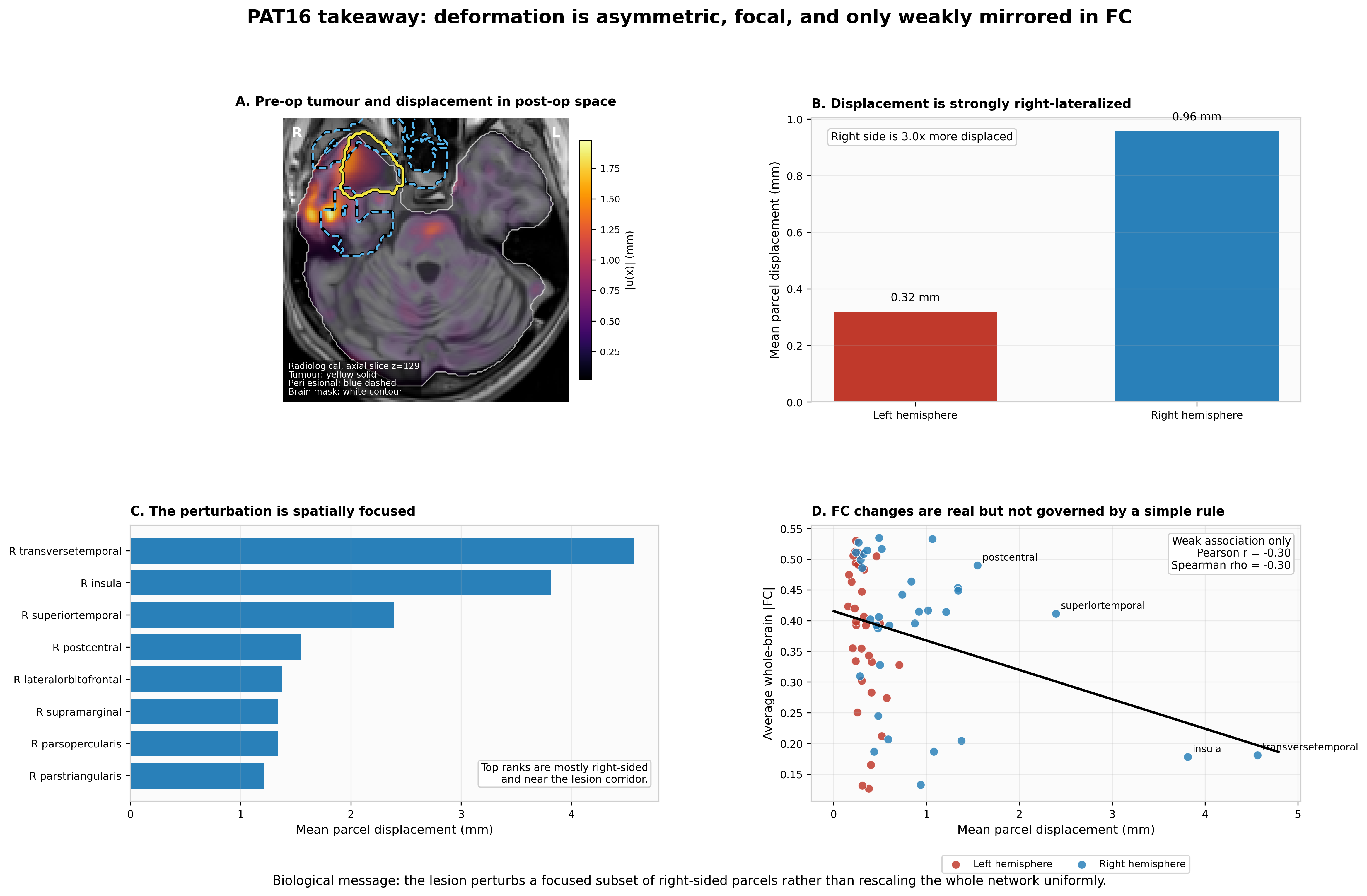
Deformation is right-lateralised and focal

Measured deformation is right-lateralised (≈ 3× the left side) and concentrated in temporal–insular parcels. FC changes relate only weakly to it (r ≈ −0.30).

Deep dive: the mechanics model

Linear elasticity on the patient mesh, with heterogeneous parameters:

\[ -\nabla\cdot\sigma(u) = f, \qquad \sigma = 2\mu(x)\,\varepsilon(u) + \lambda(x)\,(\nabla\cdot u)\,I,\qquad \varepsilon = \tfrac12(\nabla u + \nabla u^\top) \]

  • \(E(x)\) is mapped from FA and \(\nu(x)\) from MD. These mappings are heuristic.
  • Mass-effect release is modelled as a pressure \(p_0\) on the cavity boundary.
  • The measured deformation has Jacobian determinant 0.55–1.27, i.e. up to 45 % compression and 27 % expansion. That is beyond the small-strain assumption, and calls for hyperelastic or poroelastic models.

Material parameters are not fitted to this patient. Estimating them from pre/post imaging is an open inverse problem.

7 · Mechanics and neural dynamics

From deformation to network activity

  • Structural coupling: connections passing through strained tissue are weakened: \(\;SC'_{ij} = SC_{ij}\,e^{-\alpha\,\bar{s}_{ij}}\)
  • Excitability coupling: displacement shifts each region’s dynamics in a whole-brain Hopf model.
  • The model then simulates functional connectivity, which is compared with the patient’s FC.
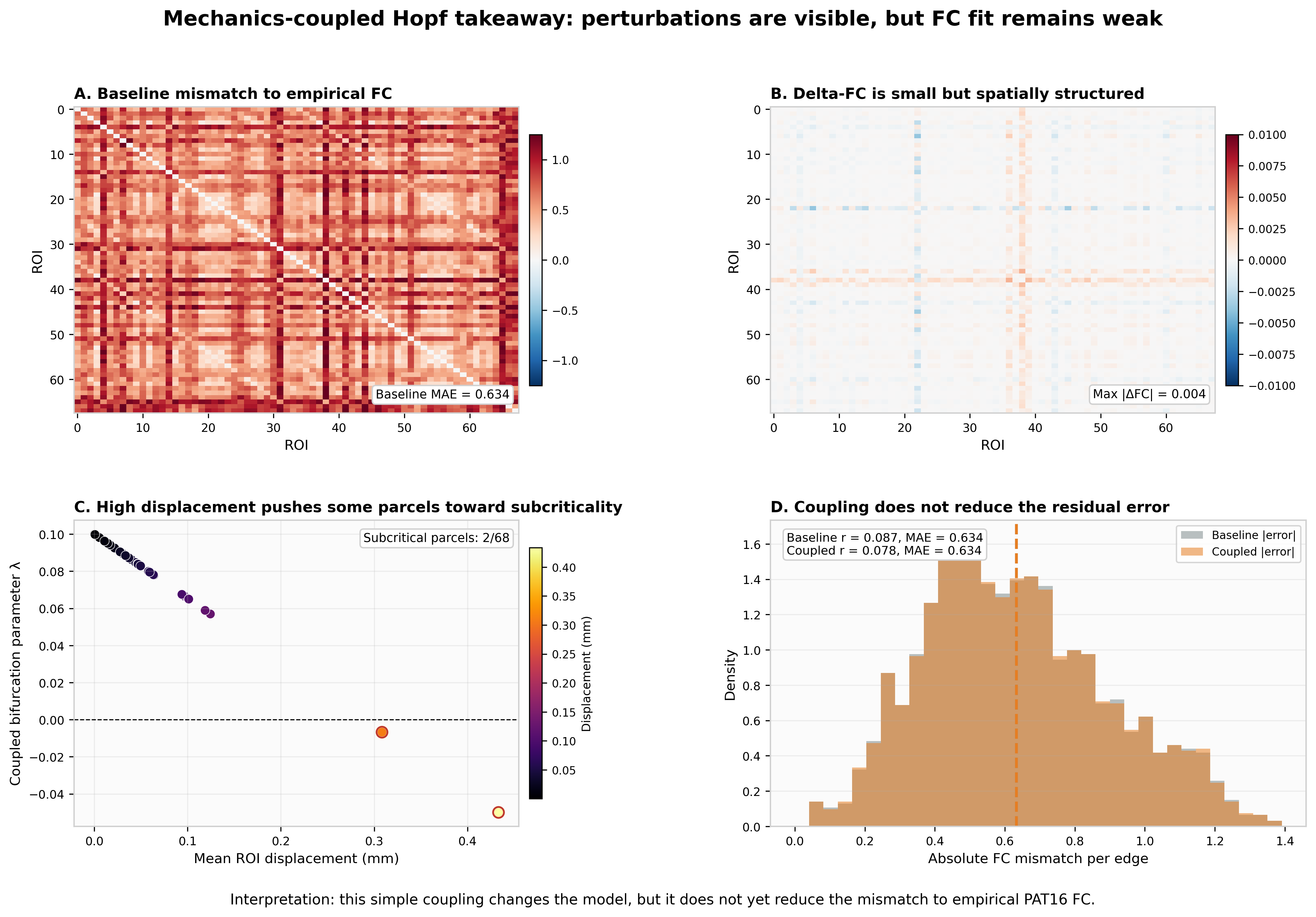
Coupled Hopf dynamics takeaway

The coupling visibly changes the simulated network. But the fit to the patient’s own FC is weak (r ≈ 0.08), and coupling does not reduce the error. The dynamics are not yet fitted to the patient.

8 · Closing the loop

Does predicted disruption match observed cognitive change?

  • Map each CANTAB domain to its supporting cortical regions.
  • Predicted vulnerability is the loss of structural connectivity in those regions after the mechanics coupling. It combines within-domain loss and loss of connections to the rest of the brain.
  • Observed change is the direction-aligned CANTAB change (positive = better).
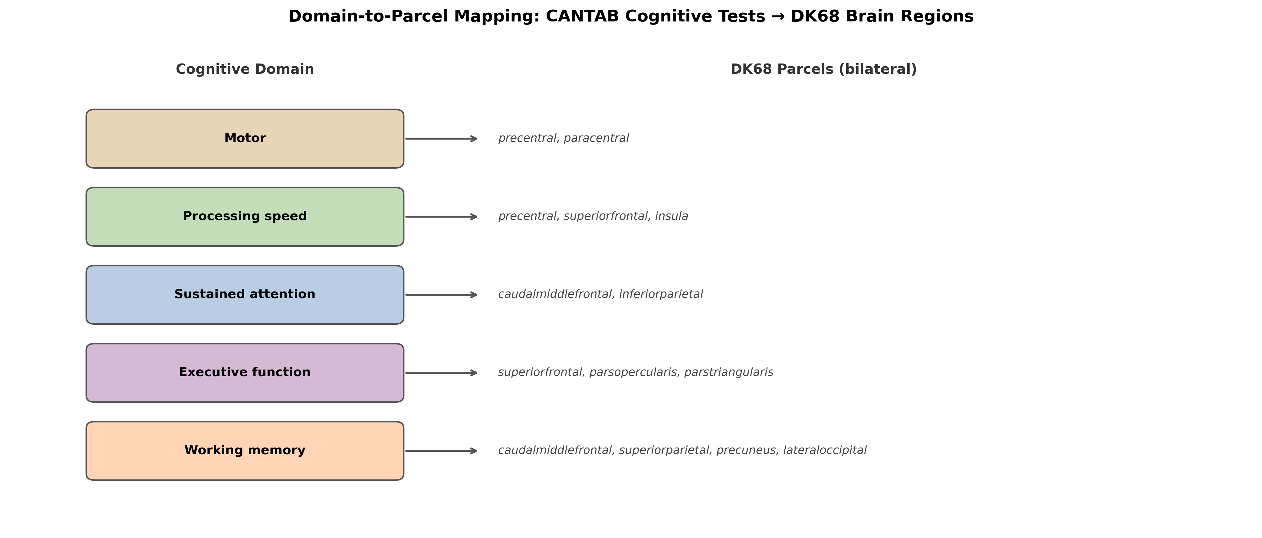
Mapping of cognitive domains to cortical parcels

The domain-to-parcel mapping is broad and literature-based. It is not patient-specific, and it does not take hemisphere into account.

Four-zone view (interactive: move the slider)

The same result as a static figure (NB_C08)
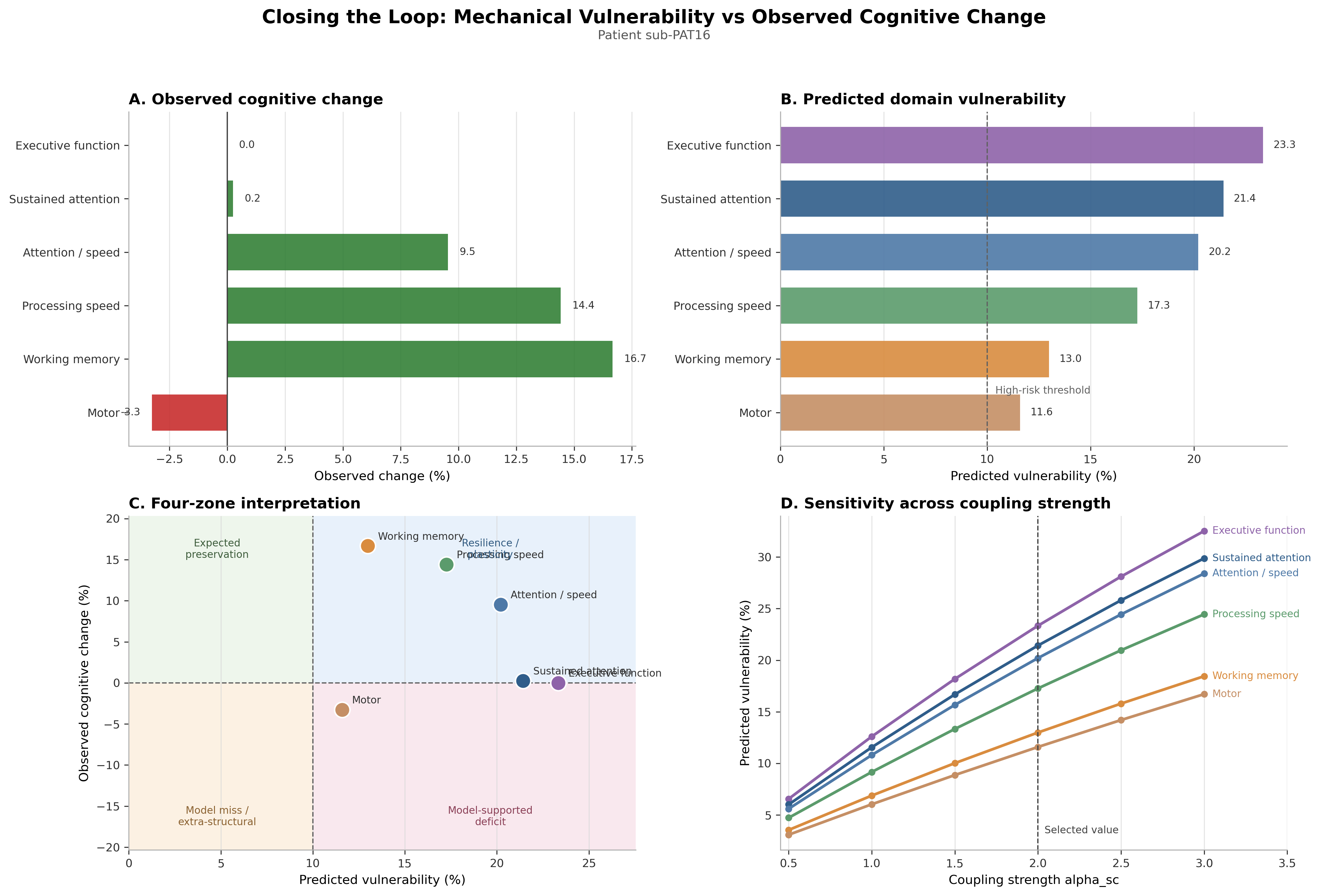
Four-panel closing-the-loop figure from notebook NB_C08

What the four-zone view tells us

Domain Predicted vulnerability Observed change Zone
Executive function (SOC) 23.3 % 0.0 % Expected preservation
Sustained attention (RVP) 21.4 % +0.2 % Expected preservation
Attention / speed (RTI 5-choice) 20.2 % +9.5 % Resilience / plasticity
Processing speed (RTI simple) 17.3 % +14.4 % Resilience / plasticity
Working memory (SSP) 13.0 % +16.7 % Resilience / plasticity
Motor (MOT) 11.6 % −3.3 % Expected preservation

What this shows: the chain from mechanics to cognition runs end to end, and mismatches become visible and discussable.

What it does not show: no observed decline exceeds 5 %, so no deficit is “confirmed”. Two sessions cannot separate real recovery from practice effects or test–retest noise.

For neuropsychologists: how to read the mismatch

Why might predicted vulnerability not show up as decline?

  • Plasticity and compensation in a slowly growing tumour
  • Practice effects on repeated CANTAB testing (RT, span)
  • Relief from mass effect and from diagnostic uncertainty (STAI ↓)
  • Raw-score change with no normative or reliable-change reference

Why might decline appear without predicted vulnerability?

  • Psychosocial burden: worry ↑, reappraisal ↓, loneliness ↑, sick leave
  • Fatigue, mood, medication, adjuvant treatment (not modelled)
  • Subcortical or white-matter effects outside the cortical parcels

Next step: use reliable-change indices and normative z-scores, add psychosocial state as explicit model variables, and test in many patients.

9 · From prototype to clinic

What is shown, and what is not yet shown

Supported by this work

  • A patient-specific twin can be assembled end-to-end from routine-type MRI plus cognitive testing.
  • Mass-effect release matters for modelling postoperative brain shift.
  • Domain-level structural vulnerability can be compared with cognition in a transparent way.
  • Psychosocial state is part of the interpretation, not noise.

Not yet supported

  • Prediction for individual patients (n = 1, retrospective)
  • Accurate mechanics: shift is underestimated, spatial agreement is poor
  • Patient-fitted dynamics: FC fit is weak
  • Uncertainty quantification across the chain
  • Comparison against simpler baselines

Roadmap to clinical translation

Stage Goal Key requirement
Now Proof-of-concept (this work) Transparent, open, reproducible pipeline
1–2 years Multi-patient validation (full BTC cohort, n = 25) Out-of-sample testing, uncertainty, baselines
3–5 years Pre-surgical prediction Does a pre-op twin predict the post-op state better than simpler models?
Vision Decision support In-silico comparison of resection or rehabilitation scenarios, with prospective evaluation

The decisive experiment is prospective: build the twin from pre-operative data only, predict the post-operative state, and compare against simple clinical models.

Mathematical challenges (deep dive)

  • Constitutive modelling: move beyond small-strain linear elasticity (hyperelastic, poroelastic, growth).
  • Inverse problems: estimate tissue and neural parameters from pre/post imaging.
  • Identifiability: decide which parameters (α, excitability shift, bifurcation λ) the data can actually constrain.
  • Uncertainty propagation: carry uncertainty from segmentation through tractography, mechanics and dynamics to cognition.
  • AI-assisted equation discovery: learn interpretable reduced dynamics from longitudinal data.

A glimpse of generative AI: “make the figure dance”

AI-generated video (Google Gemini Veo, Nov 2025) from a single photo and a text prompt.

  • A generative model animates a static scene, initialising a spatio-temporal model from one frame and a prompt.
  • Analogy for the twin: from a static pre-op scan, can we learn plausible dynamics of the patient’s brain?

Generative video is plausible, not physical. Clinical twins need mechanistic constraints and validation, not just realism.

Take-home messages

  1. A glioma brain digital twin links mechanics, networks and cognition in one patient-specific, open framework.
  2. In this patient, mechanics and dynamics are the weakest links: brain shift is underestimated and FC fit is weak.
  3. Predicted structural vulnerability did not translate into measurable decline. Resilience, practice effects and psychosocial context are all candidate explanations.
  4. The value today is transparency and testability. The next step is multi-patient, prospective validation with neuropsychological rigour.

Explore, reproduce and challenge it: github.com/arvidl/glioma-brain-digital-twin-public

Appendix

Glossary

Term Meaning
Digital twin Patient-specific computational model linked to that patient’s measured data
BIDS Brain Imaging Data Structure, a standard folder layout for neuroimaging data
DK68 Desikan–Killiany atlas: 68 cortical regions (34 per hemisphere)
SC Structural connectivity: white-matter connection strength between regions (from tractography)
FC Functional connectivity: correlation of resting-state BOLD signals between regions
FA / MD Fractional anisotropy / mean diffusivity, diffusion MRI measures of tissue microstructure
FEM Finite-element method, a numerical solution of tissue mechanics on a mesh
Hopf model Whole-brain model in which each region is an oscillator near a bifurcation point
α (alpha) Coupling strength: how strongly local strain weakens structural connections
CANTAB Cambridge Neuropsychological Test Automated Battery
Reliable change index Statistic testing whether a score change exceeds measurement error

Data, code and reproducibility

  • Repository: github.com/arvidl/glioma-brain-digital-twin-public, with the capstone notebooks NB_C01–NB_C09 (runnable in Google Colab).
  • Data: python data/download_data.py --capstone, from the OpenNeuro BTC datasets (CC0) plus project derivatives.
  • Pipeline: FreeSurfer, fMRIPrep, QSIPrep, MRtrix3, ANTs, FEniCSx, The Virtual Brain-style Hopf model.
  • This presentation: Quarto + reveal.js. The interactive figures are rebuilt from the notebooks by presentation/build_figures.py.

Licences: code MIT · text and figures CC-BY-4.0 · data CC0 (cite Aerts et al.).

References

Aerts, Hannelore, Nigel Colenbier, Hannes Almgren, et al. 2022. “Pre- and Post-Surgery Brain Tumor Multimodal Magnetic Resonance Imaging Data Optimized for Large Scale Computational Modelling.” Scientific Data 9: 676. https://doi.org/10.1038/s41597-022-01806-4.
Aerts, Hannelore, Michael Schirner, Ben Jeurissen, et al. 2018. “Modeling Brain Dynamics in Brain Tumor Patients Using The Virtual Brain.” eNeuro 5 (3). https://doi.org/10.1523/ENEURO.0083-18.2018.
Eysenck, Michael W., Nazanin Derakshan, Rita Santos, and Manuel G. Calvo. 2007. “Anxiety and Cognitive Performance: Attentional Control Theory.” Emotion 7 (2): 336–53. https://doi.org/10.1037/1528-3542.7.2.336.
Gross, James J. 2015. “Emotion Regulation: Current Status and Future Prospects.” Psychological Inquiry 26 (1): 1–26. https://doi.org/10.1080/1047840X.2014.940781.
Logothetis, Nikos K. 2008. “What We Can Do and What We Cannot Do with fMRI.” Nature 453: 869–78. https://doi.org/10.1038/nature06976.
Zarodniuk, Maksym, Anna Wenninger, Julian Najera, others, Meenal Datta, and Christopher Patzke. 2026. “Mechanical Compression Induces Neuronal Apoptosis, Reduces Synaptic Activity, and Promotes Glial Neuroinflammation in Mice and Humans.” Proceedings of the National Academy of Sciences, ahead of print. https://doi.org/10.1073/pnas.2513172122.